Testing for Independence—Pets and Sports

A survey of 325 middle school students from a city school district asks, among other things, for students’ gender, whether they prefer cats or dogs, and whether they prefer basketball or football. With these data, we can investigate whether, in this city, girls prefer cats over dogs, whether gender matters in terms of favorite sport, and whether there is a relationship between favorite pet and favorite sport.

This tutorial is not for the faint of heart; it’s a marathon. You’ll combine classic statistical inference techniques with a computer-intensive method called scrambling. You’ll simulate the null hypothesis to generate a distribution, and you’ll also plug the data into a chi-square test for independence. We’ll assume that you are familiar with the basic techniques of using Fathom.

Using a Ribbon Chart

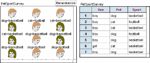
1. Open PetSportSurvey.ftm from the Tutorial Starters folder in Sample Documents. Look at the 12 cases that appear in the open collection. Simply by looking at a small number of the 325 cases in the sample, it’s impossible to make any valid predictions about what trends there might be in the whole population.

We’ll concentrate on the question of whether there is any relationship between a student’s sex and his or her pet preference.

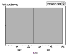
2. Make a graph and drag the Sex attribute to the horizontal axis.

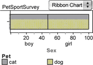
3. Change the graph to a ribbon chart by choosing Ribbon Chart from the graph’s pop-up menu. You can see from the ribbon chart the approximately equal numbers of boys and girls in the sample.

 4. Drag the Pet attribute to the middle of the graph.

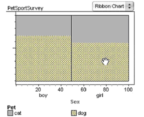
Each rectangle of the ribbon chart is now divided into two regions, one for each kind of pet. The height of the “dog” portion is higher for boys than it is for girls. This translates to “A greater proportion of boys than girls prefers dogs over cats.”        

You can use the tick marks on the vertical axis to estimate the proportion of boys that prefer dogs: a bit less that 70%. For a more exact proportion, move the mouse on top of a region in the graph and read the statement that appears in the status bar. For example, with the mouse over the girls that prefer dogs:

Computing Proportions

A ribbon chart does a good job of displaying differences in proportions. But if we want to know the computed values, we need a summary table.

5. Drag a summary table from the shelf.

6. Drag the Sex attribute to the column header of the empty summary table. 

7. Drag the Pet attribute to the row header of the table.

For a categorical attribute, a summary table shows the number of cases in each category of the attributes. We’re not interested in the counts as much as we are the proportions.

8. Double-click the formula beneath the table to show the formula editor.

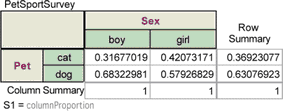
9. Type the formula “columnProportion” and click OK.

columnProportion is a special keyword that applies only to formulas for a summary table. If you oriented your table the other direction, you would want to use rowProportion.

You should see the computed column proportions for each cell. The number 0.31677019 in the cell for boys who prefer cats means that about 32% of boys prefer cats to dogs. Similarly, about 68% of boys prefer dogs to cats, whereas about 58% of girls prefer dogs to cats.

The Null Hypothesis and Choosing a Test Statistic

The heart of statistical inference is determining whether an observed difference is due to random variation or an actual difference in the population. The difference of proportions, 68% – 58%, or 10%, is fairly small. Perhaps it is due to chance. Just how likely is it that a random sample would have a difference of proportions this large if there were actually no difference in pet preferences between boys and girls?

The assumption that sex is unrelated to pet preference is the null hypothesis in this situation. Another way to phrase our question is: If the null hypothesis were true, what is the probability of getting a difference of proportions of 10% or greater? (We have to add the “or greater” because a greater difference is even stronger evidence in favor of there being a relationship between sex and pet preference.)

The difference of proportions is an example of a test statistic. Using simulation and techniques similar to those used in the tutorial, Simulation—Polling Voters, we could determine the probability of getting the observed difference of 10%. For the purposes of this tutorial, we’re going to use a closely related test statistic, called the chi-square statistic, which is commonly used for testing whether a relationship exists between two categorical attributes.

Expected Versus Observed

The chi-square statistic is based on the notion that if there were no difference between girls and boys, then the proportion of each that prefers dogs should be the same as the overall proportion of students who prefer dogs; that is, about 63%, as we can read from the row summary in the summary table. For this hypothetical sample, we would get a ribbon chart like the one at right.

Now that we know the expected proportion of boys that prefer dogs, we can compute an expected number. It is simply the expected proportion times the number of boys. Because there are 161 boys, that’s 0.63 • 161, or 101.6 boys. Similarly, for the girls, we have 63% of 164 girls, or 103.4 girls. The fractional boys and girls may seem strange, but it’s okay as long as we keep it hypothetical.

Let’s compute these numbers in the summary table.

10. Double-click the formula below the table.

11. In the formula editor, type the expression shown here and click OK. 

columnTotal, rowTotal, and grandTotal are all keywords you can use only when writing a formula for a summary table. They are in the Special list in the formula editor. You can also enter them in a formula by double-clicking them in this list. You should see the expected values computed in each cell.

Because this is such a common computation, Fathom has a shortcut for it.

12. Double-click the formula again and substitute the single word expected for the more complicated expression. (This keyword is also in the Special list.) Click OK. You should get the same results.

The term expected, or expected value, has a very general meaning in statistics. Here, in Fathom, we’re applying it to the very particular situation of a chi-square test where the null hypothesis is that the row and column attributes are independent.

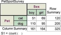
We now want to compare the expected values with the observed values.

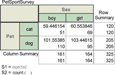
13. With the summary table selected, choose Summary | Add Formula.

14. Type the formula “count( )” into the formula editor and click OK. Your summary table should look similar to the one shown at right.

Notice that the two formulas produce the same numbers for the row and column summaries. Think about why that should be true.

Computing the Chi-Square Statistic

There are many different statistics we could invent using the observed and expected values. We’re going to use one for which statisticians have figured out how to compute a distribution without having to resort to simulation—the chi-square statistic. It’s based, as you might imagine, on the difference between the observed and expected values.

15. Add the formula shown here to the summary table. 

The chi-square statistic is simply the sum of the numbers we just computed. To calculate the sum of these values in Fathom, we have to create a collection from them.

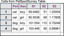
16. With the summary table selected, choose Summary | Create Collection From Cells. You should see a new collection labeled Cells from PetSportSurvey Table.

17. Make a case table for the new collection. Each case in this new collection corresponds to a single cell in the summary table—four cells and four cases. Each of the three formulas in the summary table corresponds to one attribute in the measures collection. We’re interested in the sum of the values for S3.

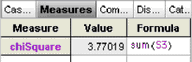18. Show the inspector for the new collection and define a measure for it, as shown at right. This number is the chi-square statistic.

We now have our statistic, but we do not yet know how likely it would be to get a chi-square value this big or bigger by chance alone. The advantage of using a well-studied statistic, however, is that Fathom can easily compute this probability for us.

19. Define a second measure, pValue, for this collection. Give it the formula shown here.

ChiSquareCumulative is a function built in to Fathom. It takes two arguments: the first is the value of chi-square that we have computed (the first measure we made); the second is the number of degrees of freedom available, in this case, 1. (If you know all the row totals and column totals, degrees of freedom is the number of cell counts you could fill in before all the rest were determined for you.) The function computes the probability of getting that value of chi-square or less under the assumption that the two attributes are independent. Because we’re interested in “or greater,” we subtract the function’s value from 1.

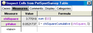
Your inspector should look similar to the one shown here. The probability of getting a chi-square statistic greater than or equal to 3.77, under the assumption of the null hypothesis, is 0.052.

What are we to make of this result? We can say that if there were no difference between boys’ and girls’ pet preferences, and if we repeated the random sampling many times, we would get a result this extreme or more extreme about 1 time in 20. For many situations, especially in the social sciences, this level of probability is persuasive enough to say that we have probably found something. But in other situations, especially in medical research, we would not be able to say we had found something, because the consequences of being wrong would be too great.

Testing for Independence—The Simple Way

You may be thinking that this was an awful lot of work to accomplish a fairly routine calculation. You’re right; and Fathom has the ability to do this computation quickly and simply. Here’s how.

You may want to hide or delete objects to free up some space. Keep the original collection and its case table.

20. Drag a test object from the shelf.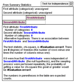 You get an empty test.

21. Choose Test for Independence from the pop-up menu.

The analysis shows #Evaluation error# for the chi-square statistics and the P–value because Fathom doesn’t yet have the information needed to compute them. We could type in the relevant values, but it’s much easier to have Fathom compute them from the raw data.

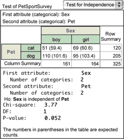
22. From the PetSportSurvey collection, drag Sex and then Pet to the top portion of the analysis.

Sometimes we don’t need a full explanation of how the inference works.

23. Choose Test | Verbose to turn off verbose mode and to see a more compact version of the test.

You should see, as shown here in the nonverbose form, the results of a chi-square test. The value of chi-square and its P-value are both given. They should be the same as the values you computed in the previous section of this tutorial.

Graphing the Chi-Square Distribution

It’s helpful to see where the computed chi-square statistic for this sample lies in the distribution of chi-square values that would result when the null hypothesis is satisfied.

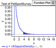
24. With the test object selected, choose Test | Show Test Statistic Distribution. The graph you get should be similar to the one shown here. The shaded area under the right portion of the curve corresponds to the P-value for the observed chi-square statistic.

Simulating the Null Hypothesis

With Fathom, we can simulate conditions under which the null hypothesis is true and repeatedly perform the sampling and computation of a chi-square statistic. Although this does not tell us anything more about the particular experiment, it does shed light on the process of statistical inference.

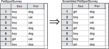
The null hypothesis states that there is no relationship between the two attributes Sex and Pet. What if we were to take all the values for the attribute Sex and scramble them so that “boy” and “girl” got reassigned randomly to each case? Any relationship that might exist between the two attributes would be wiped out by the scrambling. Any remaining relationship would have to be due to chance alone.

25. Select the PetSportSurvey collection.

26. Choose Collection | Scramble Attribute Values. A new collection should appear labeled Scrambled PetSportSurvey.

27. Make a case table for the new collection.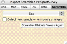

By default, Fathom scrambles the first attribute in the collection. That works well here, but in other situations you may need to scramble a different attribute. To do so, show the scrambled collection’s inspector and use the pop-up menu in the Scramble panel to choose an attribute to scramble.

28. With the scrambled collection selected, choose Collection | Scramble Attribute Values Again. You should see the values in the Sex column of the case table change each time you scramble again.

29. Make a ribbon chart for the scrambled collection, just as you did in steps 2–4.

As we scramble, we can see the variation in the relative proportions. This variation is due solely to chance.

30. Make a new test for independence. This time, drop attributes from the scrambled collection into it.

Each time you scramble again, the chi-square statistic and the P-value are recomputed. Because you’re simulating the conditions of the null hypothesis, the chi-square values will not be very large, and the P-values will not be very small.

Now we want to collect many chi-square values from the scrambled collection. We will build up a distribution of these values and see what shape it has.

31. Select the scrambled test and choose Test | Collect Results as Measures.

Fathom will scramble the scrambled collection five times, each time collecting values computed by the test for independence and putting them in a new collection, labeled Measures from Test of Scrambled PetSportSurvey.

32. Make a case table for the measures collection. Your screen should look similar to that shown below (in nonverbose mode).

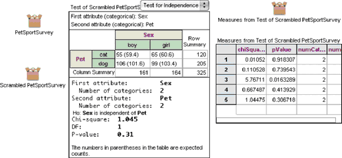
The two important columns in the table are chiSquareValue and pValue.

33. Make a histogram of each of the attributes, chiSquareValue and pValue. Your histograms won’t look like much yet, because you have only collected the results of five scrambles. You need some more.

34. Double-click the measures collection and go to the Collect Measures panel.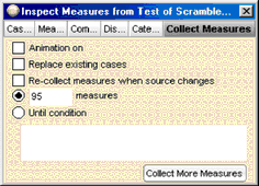

35. Uncheck both Animation on and Replace existing cases.

36. Specify that you want 95 measures instead of 5.

37. Click the Collect More Measures button.

Collecting 95 measures may take a while. A progress bar will give you an idea of how long you will need to wait. When the collection process completes, you should have 100 P-values and 100 chi-square statistics.

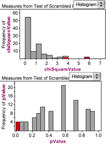
What do these histograms tell us? First, we see that chi-square statistics as high as the one we got for the original sample, 3.77, don’t occur very often. But they do occur; in fact, they occur about 5% of the time, corresponding to the P-value we computed for the original sample.

Second, the shape of the chi-square histogram markedly resembles the plotted chi-square distribution we made in step 24. That makes sense—one is from theory and the other is from simulation, but they should show the same thing.

Third, the distribution of P-values is spread over the interval from 0 to 1. Select the lowest bar in the pValue histogram and notice that the highest bars in the chi-square histogram are selected. By selecting only those P-values less than or equal to 0.05, you can read off an approximation for the so-called critical value for chi-square in the chi-square graph.

Going Further

• Consider the other two pairs of attributes possible: Sex versus Sport and Pet versus Sport. Would you expect them to show more or less independence than Sex versus Pet? Look at the corresponding ribbon charts. Do the observed differences in proportions look significant? Perform a chi-square test on each of these pairs. Explain why one result is so much more significant than the other.
• Though the ribbon chart is probably the easiest way to see relationships between categorical attributes, three other displays are possible, shown below.

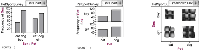
Make these three displays (using Fathom Help as needed), and learn how to interpret them. Think about circumstances in which you might prefer one versus another.