Simulation—Polling Voters
In this tutorial, you’ll simulate a population of voters, a certain proportion of whom will vote in favor of a particular proposition. You’ll investigate the question of how accurately a random sample of voters can predict the outcome of an election.
The city of Freeport has a rent control initiative, Proposition A, on the ballot. The local newspaper is going to conduct a poll three weeks before the election to gauge public sentiment. Staff members need to know how big a sample to poll. Our job is to set up a simulation they can use to determine, for any given sample size, the accuracy they should expect.
Modeling the Population of Voters
We start by creating a model for the population, the people who will vote in the election for or against the proposition. The model will consist of a single number—the proportion of voters who will vote yes.
1. Start with a new, empty document.
![]()
2. Create a slider named probYes.
A proportion can only lie between 0 and 1, so we should adjust the slider scale. We could do this by dragging on the scale until it’s close enough, but there’s another way to control axes.
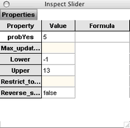
3. Double-click the slider’s axis. This brings up the slider’s inspector. The inspector lets us control the slider’s appearance and behavior.
4. Edit the values for the Lower and Upper properties (the lower and upper bounds of the axis) to be 0 and 1.
The slider models the population. We’ll use a collection to model the simulated samples. We’ll start with samples of 100.
5. Make a new collection named Sample of Voters.
6. Add 100 cases to the collection (Choose Collection | New Cases).
7. Double-click the collection.
The inspector now shows properties of the collection. There is only one inspector window. You change what it inspects by double-clicking the desired object.
8. In the inspector, create an attribute called vote by clicking <new> and typing the attribute name.
We want the values for this attribute to be “yes” and “no.” The values will be drawn from an infinite population, whose proportion of yeses is set by the slider.
9. Double-click the Formula field for the vote attribute to show the formula editor.
![]()
10. Enter the formula shown at right by typing
if(random( )<probYes Tab “yes” Tab “no”
11. Close the formula editor.
For each case, Fathom will generate a random number between 0 and 1 and evaluate it. If the number is less than the slider’s value, Fathom will give the case the value “yes”; otherwise, Fathom will give the case the value “no.” (The function random( ) has a minimum of 0 and a maximum of 1, unless you specify otherwise.)
It’s always good to check your simulations.
12. Make a case table for the collection, and check that you have a roughly even mix of yeses and noes.
13. Delete the case table.
14. Graph the vote attribute.
You should now have the three objects shown here (and the inspector).
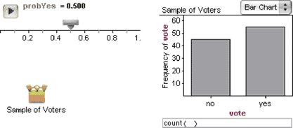
15. Choose Collection | Rerandomize several times. Each time you rerandomize, the bars in the graph change, reflecting the results of a new sample.
16. Drag the slider’s thumb to change its value to somewhere around 0.80. The vote is no longer close; it is a slam dunk for the proposition.
17. Move the slider’s thumb back to somewhere near 0.50 to model a close election.
Simulating Repeated Surveys
We now have a population whose “true vote” is controlled by a slider, and we want to see how well a sample of 100 people accurately predicts election results (compared with other sample sizes we’ll do later). We need to run the simulation many times to see how well the sampling does in the long run.
We could simply rerandomize many times, each time recording the proportion of yeses for each run (our sample statistic of interest), or we can have Fathom do this grunt work for us. In Fathom, this is called collecting measures. First, we need to define the measures to collect.
18. In the collection’s inspector, go to the Measures panel by clicking its tab.
This looks much like the Cases panel, in that there’s a prompt for creating/naming measures and a Formula column for defining how each measure is computed.
The interface for working with measures is similar to that of working with attributes, but measures themselves are different. Whereas attributes have distinct values for each case, a measure has one value for the collection as a whole.
19. Create a measure called propYesVote.
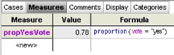
20. Give it the formula “proportion(vote = “yes”)”.
21. Check the value of the measure against the graph, and rerandomize a few times to check that your setup is working as expected.
Now that we have defined a measure, we want to collect a lot of them in a new collection (to sample our population repeatedly). Although there’s a command that will do this, let’s use the drag-and-drop method.
22. Make a new, empty collection, putting it to the right of the existing objects.

23. Drop the name of the measure onto this collection.
You’ve told Fathom to “collect this.” Fathom rerandomizes the source collection of voters, calculates the measure, and stores it in the measures collection, which is now called Measures from Sample of Voters. Little green balls fly from the source to the measures collection to help show what’s happening.
Let’s look at this collection.
24. Make a case table for the measures collection.
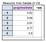
What was a measure in the source collection is now an attribute in the measures collection; each case represents the results of one survey of 100 people. We got five cases by default.
25. Graph these data.
We need to do more surveys. The controls for the measures collection are—where else?—in its inspector.
26. Double-click the measures collection to show its inspector.
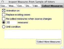
27. Go to the last panel, the Collect Measures panel.
28. Change the number of measures to collect from 5 to 20.
29. Click Collect More Measures.
The sample rerandomizes in the graph of the sample of voters, giving a new collection of votes. The proportion of yeses then appears in the graph of the measures collection.
We strongly urge leaving the animation on. The animation shows what’s happening and slows down the process. The very concept of what’s happening is hard to get at first; watching and thinking about what’s going on helps avoid confusion (for example, thinking that things in the measures collection represent some thing, rather than an abstract summary of a whole collection of things).
You might want to make a summary table of the collection of samples, showing the proportion of yeses, and run the simulation a few more times.
You could change the slider’s value, change the collect measures control to replace existing cases, and see the results of repeated polling when the race isn’t close.
But we were investigating sample size, so, when you’re finished experimenting, let’s return to that.
Changing Sample Size
The trouble is, we aren’t collecting the sample size. How do we do that? We need another measure, which we need to define for the Sample of Voters collection.
30. Double-click the collection of voters.
31. In the Measures panel, define a second measure, SampleSize, giving it the formula count().
In Fathom, the count function, without any arguments in it (such as count (sex = “male”)), simply gives the number of cases in that collection.
We need to start the simulation over, because we’re now collecting the sample sizes.
32. Double-click the measures collection, and check Replace existing cases in the Collect Measures panel.
33. Collect 50 measures. Notice that the case table first empties, and then fills with two attributes this time, one for each of the measures defined.
34. Uncheck Replace existing cases. You want to keep these measures after you change the sample size, not throw them away.
35. Select the collection of sample voters, and add 300 new cases (choose Collection | New Cases). This gives a total of 400 voters per survey.
![]()
36. Open the measures collection a little bit by dragging its bottom-right corner down and out until you can see the Collect More Measures button.
37. Click this button to collect 50 measures of samples of 400 each.
We need to add this information to our measures graph. What we want is a split dot plot.
38. Drag SampleSize from the measures collection’s case table and drop it on the vertical axis of the measures graph.
You get a scatter plot, which isn’t what you want. You need SampleSize to be treated as a categorical attribute, not a numeric one.
39. Undo the last step.
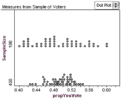
40. Drop the attribute on the vertical axis again, but this time hold down the Shift key when you drop. This forces Fathom to treat the numeric attribute as categorical, and you get a split dot plot, showing the distributions of proportions of yeses for the two sample sizes.
We now have a tool to use with the newspaper staff to show them the effects of sample size on polling results: Smaller samples have more spread than larger, for example.