Testing a Hypothesis—Plant Growth
Charles Darwin believed that there were hereditary advantages in having two sexes for both the plant and animal kingdoms. Some time after he wrote Origin of Species, he performed an experiment in his garden. He raised two large beds of snapdragons, one from cross-pollinated seeds, the other from self-pollinated seeds. He observed, “To my surprise, the crossed plants when fully grown were plainly taller and more vigorous than the self-fertilized ones.” This led him to another, more time-consuming experiment in which he raised pairs of plants, one of each type, in the same pot and measured the differences in their heights. He had a rather small sample and was not sure that he could safely conclude that the mean of the differences was greater than 0. His data for these plants were used by statistical pioneer R. A. Fisher to illustrate the use of a t-test.
Looking at Darwin’s Data
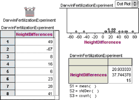
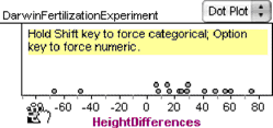
1. Open Darwin.ftm from the Tutorial Starters folder in the Sample Documents folder. This document contains the data for the experiment described above: 1 attribute, 15 cases.
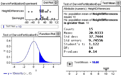
2. Make a case table, a dot plot, and a summary table similar to those shown here.
We see that most of the measurements are greater than 0, meaning that the cross-pollinated plants grew bigger. But two of the measurements are less than 0. Darwin did not feel justified in tossing out these two values and was faced with a very real statistical question.
Formulating a Hypothesis
Darwin’s theory—that cross-pollination produced bigger plants than self-pollination—predicts that, on average, the difference between the two heights should be greater than 0. On the other hand, it might be that his 15 pairs of plants have a mean difference as great as they do (21-eigths of an inch) merely by chance. You can write out these two hypotheses in Fathom in a text object to be stored with your document.
3. From the shelf, drag a text object into the document.
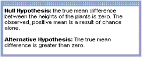
4. Write the null hypothesis and the alternative hypothesis. At right you can see one way to phrase the hypotheses.
You can choose Edit | Show Text Palette to bring up a full suite of tools for formatting text and creating mathematical expressions.
Deciding on a Test Statistic
At the time of Darwin’s experiment, there was no very good theory for dealing with a small sample from a population whose standard deviation is not known. It was not until some years later that William Gosset, a student of Karl Pearson, developed a statistic and its distribution. Gosset published his result under the pseudonym Student, and the statistic became known as Student’s t. When the null hypothesis is that the mean is 0, the t-statistic is simply, x̄/(s/√n), where x̄ is the observed mean, s is the sample standard deviation, and n is the number of observations.
Let’s compute this statistic for Darwin’s data using one of Fathom’s built-in statistics objects.
5. Drag a test object from the shelf. An empty test appears.
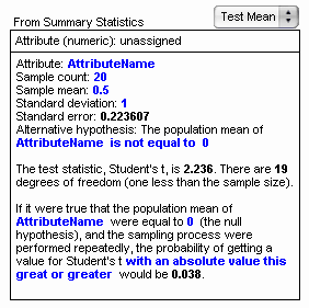
6. From the pop-up menu, choose Test Mean. As shown at right, the Test Mean test allows us to type in summary statistics. The blue text is editable. This is very useful when you don’t have raw data.
7. Try editing the blue text. You can, for example, enter the summary statistics for Darwin’s data.
Here are some things to notice.
- Changing something in one part of the test may affect other parts. For example, editing the AttributeName field in the first line also changes it in the hypothesis line and in the last paragraph.
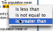
- In the hypothesis line, clicking on the “is not equal to” phrase brings up a pop-up menu from which we can choose one of three options. For Darwin’s experiment, we want the third option because his hypothesis is that the true mean difference is greater than 0. Notice that making this change alters the phrasing of the last line of the test as well.
![]()
- In addition to simple editing of numbers, we can also determine their value with a formula. For example, we might want to tie the sample count to a slider named n so that we could investigate the effect of different sample sizes. To show the formula editor, choose Edit | Edit Formula with the text cursor in the number whose value you wish to determine. These computed values display in gray instead of blue. Editing the value itself deletes the formula.
Checking Assumptions
Gosset’s work with the t-statistic relied on an assumption about the population from which measurements would be drawn, namely, that the values in the population are normally distributed. Is this a reasonable assumption for Darwin’s data?
Height measurements of living things, both plants and animals, are usually normally distributed, and so are differences between heights. But we might worry, because the two negative values give a decidedly skewed appearance to the distribution.
Fathom can help us determine qualitatively whether this amount of skew is unusual. We’ll generate measurements randomly from a normal distribution and compare the results with the original data.
8. Make a new attribute in the collection. Call it simHeight for simulated height.
9. Select simHeight and choose Edit | Edit Formula. Enter the formula shown below.
![]()
This formula tells Fathom to generate random numbers from a normal distribution whose mean and standard deviation are the same as in our original data. We want to compare the distribution of these simulated heights with the distribution of the original data. We can do that directly in the dot plot that already shows HeightDifferences.
10. Drop simHeight on the plus sign to add it to the horizontal axis. The graph now shows the original data on top and the simulated data on the bottom.
One set of simulated data doesn’t tell the whole story. We need to look at a bunch.
11. Choose Collection | Rerandomize.
Each time you rerandomize, you get a new set of 15 values from a population with the same mean and standard deviation as the original 15 measurements. Three examples are shown below.
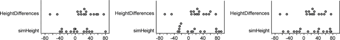
A bit of subjectivity is called for here. Does it appear that the original distribution is very unusual, or does it fit in with the simulated distributions?
Testing the Hypothesis
Once we have decided that the assumption of normality is met, we can go on to determine whether the t-statistic for Darwin’s data is large enough to allow us to reject the null hypothesis.
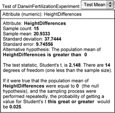
In step 7, we typed the summary values into the test as though we didn’t have the raw data. But we are in the fortunate position of having the raw data, so we can ask Fathom to figure out all the statistics using that data.
12. Drag HeightDifferences from the case table to the top pane of the test where it says “Attribute (numeric): unassigned.”
13. If the hypothesis line does not already say “is greater than,” then select that choice from the pop-up menu.
The last paragraph of the test describes the results. If the null hypothesis were true and the experiment were performed repeatedly, the probability of getting a value for Student’s t this great or greater would be 0.025. This is a pretty low P-value, so we can safely reject the null hypothesis and, with Darwin, pursue the theory that cross-pollination increases a plant’s height compared with self-pollination.
Looking at the t-Distribution
It is helpful to be able to visualize the P-value as an area under a distribution.
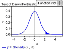
14. With the test selected, choose Test | Show Test Statistic Distribution. The curve shows the probability density for the t-statistic with 14 degrees of freedom. The shaded area shows the portion of the area under the curve to the right of the test statistic for Darwin’s data. We’ve set this up as a one-tailed test; we’re only interested in the mean difference being greater than zero. The total area under the curve is 1, so the area of the shaded portion corresponds to the P-value for Darwin’s experiment.
Let’s investigate how the P-value depends on the test mean, which is currently set to 0.
15. Drag a slider from the shelf into the document.
16. Edit the name of the slider from V1 to TestMean.
17. Select the 0 in the statement of the hypothesis in the test. Choose Edit | Edit Formula.
18. In the formula editor, enter the slider name TestMean and click OK.
Now the value of the null hypothesis mean in the test and the shaded area under the t-distribution change to reflect the new hypothesis.
19. Drag the slider slowly and observe the changes that take place.
For what value of the slider is half the area under the curve shaded? Explain why it should be this particular value.
The illustration below shows something similar to what you probably
have. Note that the test has been switched to “nonverbose” (choose
Test | Verbose).
Going Further
- Play around with changing the data and observing the effect on the P-value. How much closer to 0 can the experimental mean be (without changing the standard deviation) and still have a P-value greater than 0.05? If you make the standard deviation smaller, what happens to the P-value (and why)?
- Make a Test Mean object that tests the mean of simHeight instead of HeightDifferences. Notice that each time you rerandomize, you get a new P-value. Think about what it means when the P-value is greater than 0.05. Would you call this a “false positive” or a “false negative”? By repeatedly rerandomizing, estimate the proportion of the time that the P-value is greater than 0.05. What practical significance would that have in planning an experiment?