Generating Mathematics—Change Playground

This tutorial also focuses on using formulas to define new attributes, but this time you’ll work in a purely mathematical context, experimenting with change and how to calculate change using Fathom’s “prev” function.

Creating the Collection

Here, we don’t have data in the sense of observations; rather, we are working simply with some numbers.

1. In a new, empty document, make a new case table with two attributes: A and B.

2. Give attribute A the values 1, 2, 3, 4, and 5.

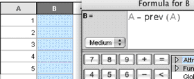
3. Select attribute B, and choose Edit | Edit Formula to show the formula editor.

4. Type “A–prev(A)”.

You are telling Fathom to compute values for B defined as the difference between each case’s value for A and the previous case’s value for A. Before accepting the formula, you predict what each value of B will be. Why?

5. Click OK to accept the formula and close the formula editor.

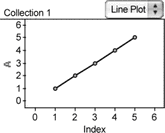
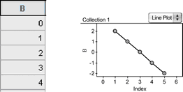
6. Make a line plot of A by putting A on the vertical axis of a new graph and choosing Line Plot from the graph’s pop-up menu. The horizontal axis is now labeled Index (the first case has a caseIndex of 1; the second, 2; and so on).

7. Similarly, make a line plot of B.

Just for fun, let’s make the dots bigger in these two graphs.

8. Double-click the A graph’s axis.

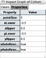
This shows the graph’s inspector.

The inspector lets us control properties of the graph. For example, instead of dragging axes to rescale a graph, we can numerically specify the upper and lower bounds of an axis: xLower and xUpper control the horizontal axis’s lower and upper bounds.

9. In the inspector, change the value for pointSize to 8. All the data points in this graph are bigger.

10. Double-click an axis in the B graph. The inspector shows the properties of the B graph.

11. Change B’s pointSize to 8.

12. Close the inspector by clicking its close box.

Playing with Change

13. In the graph of A, drag point 3. You will see the value changing in the case table. The graph of B will also change. What points in B move? How do they move? Why?

14. Try to drag a point in B. You can’t change these values by dragging, because they are defined by formula.

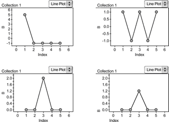
15. Change the data in A to 10, 8, 6, 4, and 2.

16. If necessary, rescale each graph so that all the points show again, by selecting the graph and choosing Graph | Rescale Graph Axes.

What does graph B show? Why does it show this?

The screen shots below each show a set of data of B. Create each graph or table on your computer by changing the data for A.

Cumulative Sum

Let’s make a new attribute, C, that is the cumulative total of A for each case.

17. Add the attribute C, giving it the formula A + prev(C).

Note that it’s not A + prev(A), because that would add only two values of A, rather than adding to the previous cumulative sum of A.

18. Make a line plot of C. What shape is this? Why? (There’s a calculus connection here: B is the derivative of A; C is the integral.)

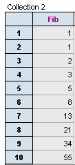
Fibonacci Numbers

Now that we’re used to how the prev function works in Fathom (there’s also a next function that takes the value of the next case), we can look at other uses, such as the Fibonacci numbers (1, 1, 2, 3, 5, 8, …). For this, we’ll start over, making another collection.

19. Scroll down in the Fathom window to give yourself a blank area.

20. Make a new, empty case table with an attribute called Fib.

We need to use a formula that will result in the first two cases getting the value 1 and the rest of the cases getting the sum of the previous two numbers. For this, we need an if-statement.

21. Select Fib and choose Edit | Edit Formula.

22. Type “if(“.

When you type the open parenthesis, Fathom gives you a template for filling out the if statement. You want the first two cases to have the value 1.

23. Inside the parentheses, type “caseIndex≤2”. (To get the “≤” symbol, press Ctrl (Win) or Option (Mac) and click the < button that appears on the keypad.)

24. Press Tab to get to the top result clause. (This specifies what value the cases that meet the condition get.)

25. Type “1” and tab to the next clause.

For all cases that don’t meet the specified condition, we want the result to be the sum of the two previous values.

26. Type “prev(Fib) + prev(prev(Fib))”.

So, the whole formula says, for the first two cases, give a value of 1; otherwise take the previous value and add it to the value before that. This construction is typical for a recursive definition: Use caseIndex in an if statement to define the initial condition. One fork of the if statement defines the initial values; the other defines the recursive step.

27. Close the formula editor.

The case table is still empty, because you haven’t added any cases to this collection (in the past, you simply typed them).

28. Select the collection (the box of gold balls labeled Collection 2), and choose Collection | New Cases.

29. Type “10” and click OK. The case table fills with the results of your formula.

30. Make a line plot of Fib.

31. Add an attribute n to the case table, giving it the formula CaseIndex. Now the case numbers appear as an attribute (not simply as row labels in the case table).

32. Put n on the horizontal axis of the graph.

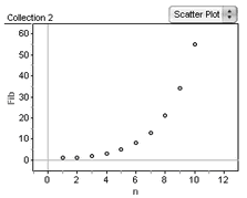
If you like, you could go on to fit a function to this graph. You could also add more cases to the collection and explore what happens to the ratio of adjacent values of Fib as n increases.